Cluster Time Series Data with PCA and DBSCAN

In this article, we explore the clustering of time series data using principal component analysis (PCA) for dimensionality reduction and density-based spatial clustering of applications with noise (DBSCAN) for clustering. This technique identifies patterns in time series data, such as traffic flow in a city, without requiring labeled data. We use Intel® Extension for Scikit-learn* to accelerate performance. Time series data often exhibit repetitive patterns due to human behavior, machinery, or other measurable sources. Identifying these patterns manually can be challenging. Unsupervised learning approaches like PCA and DBSCAN enable us to discover these patterns.

Methodology

Data Generation

We generate synthetic waveform data to simulate time series patterns. The data consists of three distinct waveforms, each with added noise to simulate real-world variability. We use the scikit-learn* agglomerative clustering example authored by Gaël Varoquaux (figure 1). It is available under BSD-3Clause or CC0 licenses.

import numpy as np 
import matplotlib.pyplot as plt 
 
np.random.seed(0) 
n_features = 2000 
t = np.pi * np.linspace(0, 1, n_features) 
 
def sqr(x): 
   return np.sign(np.cos(x))
 
X = [] 
y = [] 
for i, (phi, a) in enumerate([(0.5, 0.15), (0.5, 0.6), (0.3, 0.2)]):  
   for _ in range(30):  
      phase_noise = 0.01 * np.random.normal()  
      amplitude_noise = 0.04 * np.random.normal()  
      additional_noise = 1 - 2 * np.random.rand(n_features)  
      additional_noise[np.abs(additional_noise) < 0.997] = 0  
      X.append(12 * ((a + amplitude_noise) 
                  * (sqr(6 * (t + phi + phase_noise))) 
                  + additional_noise))  
      y.append(i)
  
X = np.array(X) 
y = np.array(y)
 
plt.figure() plt.axes([0, 0, 1, 1]) 
for l in range(3): 
   plt.plot(X[y == l].T, alpha=0.5, label=f’Waveform {l+1}’) 
plt.legend(loc=’best’) 
plt.title(‘Unlabeled Data’) 
plt.show()

Figure 1. Code and plot generated by the author from scikit-learn agglomerative clustering algorithm developed by Gaël Varoquaux.

Accelerate PCA and DBSCAN with Intel® Extension for Scikit-learn*

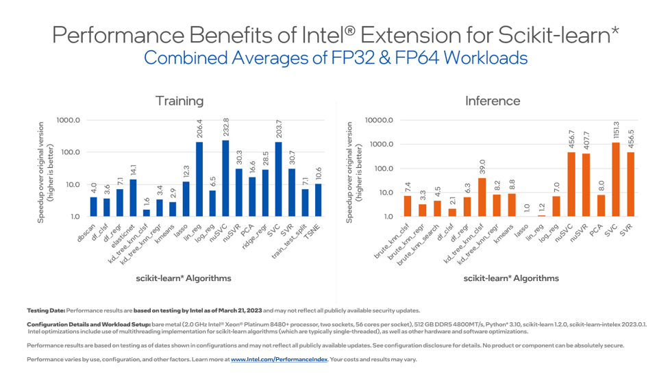
Both PCA and DBSCAN can be accelerated via a patching scheme using Intel Extension for Scikit-learn. Scikit-learn is a Python* module for machine learning. Intel Extension for Scikit-learn is one of the AI Tools that seamlessly accelerates scikit-learn applications on Intel CPUs and GPUs in single- and multi-node configurations. This extension dynamically patches scikit-learn estimators to improve machine learning training and inference by up to 100x with equivalent mathematical accuracy (figure 2).

Figure 2. GitHub* repository for Intel Extension for Scikit-learn

Intel Extension for Scikit-learn uses the scikit-learn API and can be enabled from the command line or by modifying a couple of lines of your Python application prior to importing scikit-learn:

from sklearnex import patch_sklearn 
patch_sklearn()

Dimensionality Reduction with PCA

Before attempting to cluster 90 samples, each containing 2,000 features, we use PCA to reduce dimensionality while retaining 99% of the variance in the dataset:

from sklearn.decomposition import PCA  

pca = PCA(n_components=4) 
XPC = pca.fit_transform(X)  

print("Explained variance ratio:", pca.explained_variance_ratio_) 
print("Singular values:", pca.singular_values_) 
print("Shape of XPC:", XPC.shape)

We use a pairplot to look for visible clusters in the reduced data (figure 3):

import pandas as pd 
import seaborn as sns 
 
df = pd.DataFrame(XPC, columns=[‘PC1’, ‘PC2’, ‘PC3’, ‘PC4’]) 
sns.pairplot(df) 
plt.show()

Figure 3. Looking for clusters in the data after dimensionality reduction

Cluster with DBSCAN

Based on the pairplot, PC1 and PC2 seem to separate the clusters well, so we use these components for DBSCAN clustering. We can also get an estimate of the DBSCAN EPS parameter. I chose 50 because the PC1 versus PC0 diagram suggests that this is a reasonable separation distance for the observed clusters:

from sklearn.cluster import DBSCAN  

clustering = DBSCAN(eps=50, min_samples=3).fit(XPC[:, [0, 1]]) 
labels = clustering.labels_  

print("Cluster labels:", labels)

We can plot the clustered data to see how well DBSCAN has identified the clusters (figure 4):

plt.figure() 
plt.axes([0, 0, 1, 1]) 
colors = ["#f7bd01", "#377eb8", "#f781bf"]

for l, color in zip(range(3), colors): 
 plt.plot(X[labels == l].T, c=color, alpha=0.5, label=f’Cluster {l+1}’)

plt.legend(loc=’best’) 
plt.title(‘PCA + DBSCAN’) 
plt.show()

Figure 4. Plot of clustered data generated using the previous code example

Compare to Ground Truth

As you can see from figure 4, the DBSCAN does a good job finding plausible colored clusters and compares well to the original ground truth data (figure 1). In this case, the clustering recovered the underlying patterns used to generate the data perfectly. By using PCA for dimensionality reduction and DBSCAN for clustering, we can effectively identify and label patterns in time series data. This approach allows for the discovery of underlying structures in the data without the need for labeled samples.